Straight Away to Orion
Video not displaying? Click here:
- Project 2: http://www.youtube.com/watch?v=QKCsvtl99lY
- Project 4: http://www.youtube.com/watch?v=L8rUgxSiljE
Jump to Section
-
Data
-
Application
-
Graph Modification
-
Source Code
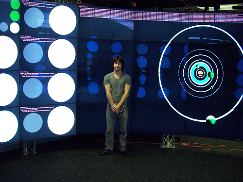
Application Running in CAVE2
 |
 |
Data
Source
The data was taken from the Open Exoplanet Catalogue.
There are two directories of XML files, “systems” and “systems_kepler”, where “systems” contains confirmed planets and “systems_kepler” objects of interest.
The application makes use of all the XML files from “systems” which contains 731 solar systems, 800 stars, and 983 planets as of the time of download.
Among these systems are single star solar systems (such as our solar system), binary, trinary, and 1 quadrinary solar system.
Each solar system is specified with <system>, <binary>, <star>, and <planet> tags that each contain tags of data specific to each kind of object.
A description of all tags in the XML files can be found here.
Manipulation
The XML files from the Open Exoplanet Catalogue were modified to be easily read programmatically.
In addition there were some minor mistakes both informationally and syntactically that were changed in the files.
As I did not want to write a general purpose XML reader for the project, I’ll describe the process of reading the data.
-
allFilesIntoOne.py
A Python script was written that reads the content of each file in the “systems” directory. The content is concatenated into one large file named “allSystems.xml”
-
removeFromXML
Another Python script was written that searches “allSystems.xml” for specific tags and creates a new XML file with these tags omitted. The purpose of this script was originally to reduce the amount of information but also simplifies programmatically reading the data as all tags become single line (some spanned multiple lines). The following tags were removed:
-
<image>
The images did not exist in the download originally. After posting an issue, the contributor added the images of the planets also mentioning: “We moved the images to a separate repository because the repository became rather larger and the images are not very helpful for any scientific purpose”. The images were not the sphere textures I was hoping for, they were invented representations of the planets. - <imagedescription>
-
<list>
The list tag had the information “Confirmed planets” for every system and so I the information was not helpful to me. Some of the binary systems differentiated between “P” and “S” systems. - <magB>
- <magI>
- <magJ>
- <magH>
- <magK>
- <videolink>
-
<image>
-
Error Reformatting
Many of the tags specify error values as attributes for the data and typically specified as errorminus or errorplus. Some of these tags did not have a value, only error specifications and so tags in the format <tagname someerror=“somevalue”/> were manually rewritten:
- Tags like <tagname upperlimit=“somevalue”/> were rewritten as <tagname errorminus=“somevalue” errorplus=“0.0”>somevalue</tagname>.
- Tags like <tagname lowerlimit=“somevalue”/> were rewritten as <tagname errorminus=“0.0” errorplus=“inf”>somevalue</tagname>.
-
Binary Formatting
The application creates a hierarchical structure of the objects in the XML file and each is a separate Python class. This process is greatly simplified by the simple data transformation below and so it was done whenever applicable among the 71 <binary> tags:
-
A structure such as:
<system><binary></system><star></star></binary>
<binary><star></star></binary>
<star></star> -
Became:
<system><binary></system><binary></binary><star></star></binary>
<star></star>
<star></star>
-
A structure such as:
-
Tag <name>
Every object had a at least one <name> tag with the exception of binaries. The following changes were made to the <name> tags of “allSystems.xml”:
- There was only one binary that had a <name> tag and so it was removed (it was redundant with its parent’s name from the point of view of the application).
- BD-061339 and HIP 27803 are <name> tags in two different systems. It seems that it was mistakenly included in Gliese 221 / GJ 221 as these are the only <name> tags for the other system. In addition, any name starting with BD-061339 or HIP 27803 was removed from the star and planets of Gliese 221 / GJ 221.
- Some <name> tags were capitalized for lexicographic order (for example: “o Serpentis” became “O Serpentis”).
- Some <name> tags were redundant and removed (for example: “gamma Cephei” is redundant with “Gamma Cephei”).
XML to Python
The overall process in converting the XML data to programmatic information involved creating a stack of the tags <system>, <binary>, <star>, and <planet> while reading line by line from “allSystems.xml”.
All tags found after pushing the stack were logically associated with the last element on the stack.
When the corresponding </system>, </binary>, </star>, or </planet> tag is found, the stack is popped and an appropriate Python class instance is made with the logically associated tags.
The Python classes directly associated to this process are:
-
System
Has Binary, Star, and / or Planet class instances as children. Instances have no parent or geometry and generally serves the purpose of being a logical root in a multi-class tree structure.
-
Binary
Has Binary, Star, and / or Planet class instances as children and System or another Binary as a parent. Instances have no geometry directly associated with but reposition child class instance geometry if the associated <binary> tag had <semimajoraxis> and / or <period> tags.
-
Star
Has Planet class instances as children and System or Binary as a parent. Instances have logical control over a transparent sphere and a light (geometry is shared among different systems) both colored based on the associated <star> tag’s <spectraltype> tag. In addition geometry for the habitable zone associated with the <star> tag is associated with this class.
-
Planet
Has no children and System, Binary, or Star class instances as a parent (orphan planets have a System parent). Instances have logical control over a sphere and line set (geometry is shared among different systems) based on the associated <planet> tag’s <radius> and <semimajoraxis>.
Application
Additional Data
The amount and type of data collected from “allSystems.xml” was not sufficient for representation of many systems as a lot of it is missing.
Additional data is created based on what data the Python classes have:
-
Binary
- Semi-minor axis can be found given semi-major axis and eccentricity.
- If period data exists it is inverted (1.0/period).
-
Star
- Radius can be found given mass.
- Logical geometry / light color associated to Star instance spectral type attribute.
- Habitable zone can be found given (root parent System) distance, magV, and spectral type.
- Habitable zone “backup plan” by table lookup (if there is not enough information for the first method) given spectral type.
-
Planet
- Radius by table lookup given mass.
- Period or semi-major axis given semi-major axis or period.
- Semi-minor axis can be found given semi-major axis and eccentricity.
- If period data exists it is inverted (1.0/period).
System Representations
 |
 |
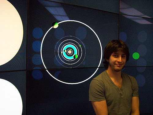
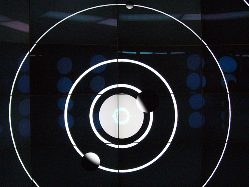
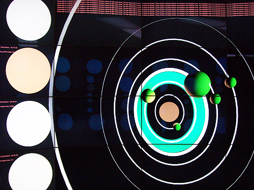
When the application begins it displays the “Sun” system in the center third of CAVE2. The “Sun” (and Star instances in general) are represented by a transparent sphere and a light both with the apparent color given its spectral type (unknown / invalid spectral types are represented with green stars). The planets (Mercury, Venus, Earth, etc.) are represented by opaque white spheres. Because omegalib lights affect the white opaque spheres, geometry associated with Planet instances gain the light from the Star instances in the system and are appropriately black where there is no light. Planet instances also have associated line set geometry which show their elliptical orbit path (with the exception of orphan planets). Finally, the habitable zone of each Star instance is represented by a line set.
Due to the extreme differences involved with the data relative to objects within different systems time, distances, and sizes are all linearly normalized:
-
Time
The periods of Binary and Planet instances were inverted during the Additional Data step. The significance of having done this is that the object with the largest period in days now has the lowest value for period. Taking the maximum of the Binary and Planet instance periods and dividing by 2.0*π results in a value I will refer to as maxOrbit. Dividing the inverted periods by maxOrbit results in the fastest object making one complete orbit per second and the other objects maintaining their orbit speed relative to the fastest.
-
Binary Distance
The semi-major axii of Binary instances are normalized by finding the maximum value. However, a value of 1.0 is too small for visual representation and so it is scaled up 1 order of magnitude to 10.0 (the largest Binary instance in a system has a semi-major axis of 1.0).
-
Star Size
The radii of Star instances are normalized by finding the maximum value (the largest Star instance in a system has a radius of 1.0).
-
Planet Size
The radii of Planet instances are normalized by finding the maximum value (the largest Planet instance in a system has a radius of 1.0).
- Planet Distance The semi-major axii of Planet instances are normalized by finding the maximum value. However, a value of 1.0 is too small for visual representation and so it is scaled up 1 order of magnitude to 10.0 (the largest Planet instance in a system has a semi-major axis of 1.0).
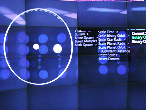
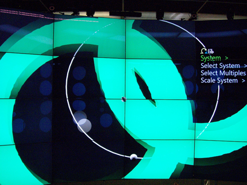
In addition the user has control over multipliers to the normalized categories through the “Scale System” menu. Each of the categories above can be manipulated for further visual tweaking.
Distinguishing from binary and planetary distances causes an impossible representation but it is useful visually as everything can be placed on the screen at a reasonable size. However, representing the habitable zone now becomes impossible as distinguishing between types of distance is problematic. To resolve this issue, a “Constant Distance” mode can be enabled from the “Scale System” menu. When this mode is active the semi-major axii of Binary and Planet instances are considered at the same time resulting in constant distance. The drawback of this mode is that it tends to cause a mess visually and requires substantial effort from the user to manipulate scale from the “Scale System” menu. On a side note, manipulating Binary Distance or Planet Distance in “Constant Distance” mode affects both scales.
System Notifications
 |
 |
There are two containers positioned above the System Representations area, the “Description” and “Missing Data” containers. The original XML files had description tags for some of the planets giving general information. When a System instance is selected any general information is displayed at the top left in the “Description” container (if there is not general information the container is invisible). If the System instance’s children are missing data and cannot be displayed then the this is mentioned at the top right in the “Missing Data” container (otherwise the container is invisible). In addition, any Star instance that has insufficient data to represent its habitable zone will give a notification in the “Missing Data” container. All items in the “Missing Data” container display the available data that objects have showing why they could not be represented.
Multiples
 |
 |
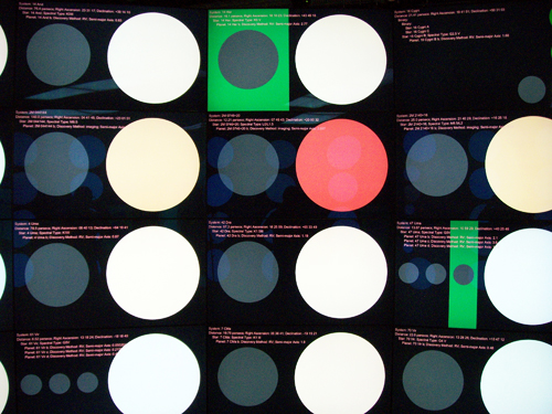
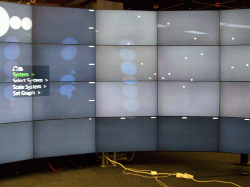
The left and right thirds of CAVE2 are dedicated to the multiples, semi-transparent containers with opaque information about the System instances. There are 24 multiples per side (48 total) and each represent one System instance of the 731 from “allSystems.xml” into 31 pages (int(ceil(731/24)) == 31). Control over what page either side of CAVE2 is displaying is done through the “Select Multiples” menu but by default the left side displays page 0 and the right side page 15. Interaction between the wand and multiples is supported by converting wand rays into 2D coordinates and performing a hit test on each multiple container. As the wand passes over multiple containers, the one with a “True” hit test is highlighted and selecting it with the D-Pad Up button loads the associated System instance into the System Representations area. The actual conversion of omegalib wand rays to 2D coordinates is performed by the “CoordinateCalculator.py” module.
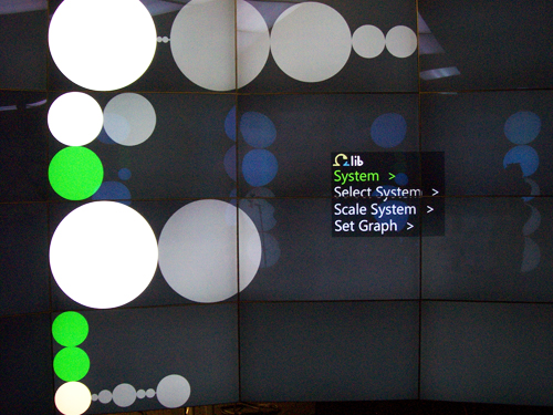
Each multiple shows an abstraction of the System instances on one CAVE2 display screen. Single star systems are shown by a large circle (one CAVE2 display screen height diameter) of the color associated with the Star instance’s spectral type (unknown / invalid spectral types are represented with green stars). Binary star systems have two medium sized circles (each half one CAVE2 display screen height diameter), trinary star systems three small circles (each a third one CAVE2 display screen height diameter), and all stars have the color associated with the Star instances’ spectral type. To the left of each Star instance are the Planet instances represented by gray circles and the number of gray circles corresponds to the number of children a Star instance has. If a Star instance has a habitable zone with Planet instances inside it (semi-major axis is within the habitable inner and outer radius) then that planet is highlighted by a green rectangle.
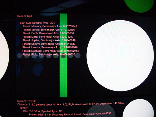
All of the above information is meant to be visually simple and designed for quickly scrolling through pages of System instances. The hierarchical and numerical information is shown at the top left corner of each multiple. This section contains all relevant available data for each of the System, Star, and Planet instances (Binary instances are mentioned only for hierarchical purposes). It is expected that a user wanting more information about a particular multiple would select it to display it in the System Representations area.
Graph Modification
Overview
 |
 |
Note: The multiples were not reasonably modifiable to be used with the graph and their original code was completely removed. Features they had in controlling System instance selection, menu options, and their own display elements do not exist in this version.
A modification to the project was created allowing System instances to have their data shown in a graph. Although the data existed in the project originally, it was only displayed as text within the multiples making comparisons difficult. Originally the multiples visually represented the number and color of Star instances, the number of Planet instances within a multiple, and Planet instances within a Star’s habitable zone if any. Multiples were modified to show the relative Planet instance radii and absence of a Star instance parent. This was intended to also assist in the main System instance visualization as all values it uses are normalized.
Features
Initially the graph has one child multiple, the “Sun” System instance.
When multiples are selected they become a child of the graph and have their user defined data represented.
If the graph would inherit more than 4 children then the oldest child (that is not the “Sun” System instance) is removed.
Each of a multiple’s Planet instances are represented by a point the color of its parent Star instance’s spectral type.
If a Planet instance’s parent is not a Star instance or the spectral type is unknown it is represented in green.
Both the x-axis and y-axis can be controlled through the menu and each have the following options:
In addition either axis may be set to consider values linearly or logarithmically if applicable (ignored for Equal Spacing and Detection Method). Linear representation is simple, the maximum is found among the appropriate class instance’s value for all children in the graph, each value is normalized with the maximum, and then mapped onto the graph. Logarithmic representation is considerably more complicated and follows this process to avoid manipulating the data incorrectly:
Both the x-axis and y-axis can be controlled through the menu and each have the following options:
-
Equal Spacing
This option is the default for both the x-axis and y-axis causing a diagonal line initially. It is an independent option in that each multiple’s Star instances do not consider other graph children Star instances for display. It serves the purpose of convenience rather than actual data as it simply separates the points representing Planet instances equidistantly along one axis.
-
Detection Method
A dictionary of all possible discovery methods is created (including unknown) and used to separate Planet instances into discrete zones. Each Planet instance is considered independently of the others.
-
Star Distance to the Sun
The database maintains this information at a System instance level and so all Planet instances within a multiple will have the same value. This option is not independent as the positioning of a point is based on the maximum of all graph children’s System distance.
-
Planet Distance from its Star
The database maintains this information at a Planet instance level and so each point in the graph may be unique.
-
Planet Eccentricity
The database maintains this information at a Planet instance level and so each point in the graph may be unique.
-
Planet Mass
The database maintains this information at a Planet instance level and so each point in the graph may be unique.
-
Planet Orbital Period
The database maintains this information at a Planet instance level and so each point in the graph may be unique.
-
Planet Radius
The database maintains this information at a Planet instance level and so each point in the graph may be unique.
-
Stellar Magnitude
The database maintains this information at a Star instance level and so all Planet instances parented to that Star instance will have the same values. This option is not independent as the positioning of a point is based on the maximum of all graph children’s Star magV.
In addition either axis may be set to consider values linearly or logarithmically if applicable (ignored for Equal Spacing and Detection Method). Linear representation is simple, the maximum is found among the appropriate class instance’s value for all children in the graph, each value is normalized with the maximum, and then mapped onto the graph. Logarithmic representation is considerably more complicated and follows this process to avoid manipulating the data incorrectly:
- Loop through all values storing them as well as the maximum.
- If the maximum is not equal to 1.0, find the log of the value and the maximum, then normalize. If the maximum is 1.0 only the log of the value is stored to avoid a division by zero. If the maximum was less than 1.0 then the logarithmically normalized value must be inverted.
- The previous step can produce negative values and so the minimum is found for all values. If the minimum is less than 0.0 then each value has this subtracted from it (so that the new minimum among them becomes 0.0). The maximum is found again for the new values as they may extend past 1.0 and each value is normalized against this new maximum.
Source Code
Instructions
-
Project 2
All files needed to run the project AlexSystems.zip. Open the Terminal, navigate to the downloaded directory, and type orun -s alexSystems.py.
-
Project 4
All files needed to run the project AlexSystems2.zip. Open the Terminal, navigate to the downloaded directory, and type orun -s alexSystems2.py.
Credits
- This project makes use of omegalib and its modules to navigate and display geometry.
- The module “CoordinateCalculator.py” is used for wand ray to 2D coordinate interaction (conversion code for manipulating multiples with the wand).